Show Me the Code!
# install packages
install.packages("sf")
install.packages("terra")
install.packages("lidR")
install.packages("viridis")
install.pacakges("future")To successfully work your way through this exercise requires that you have: (1) a working computer with at least four cores, at least 8GB of RAM, at least 2GB free storage (local or network); (2) R installed (the exercise is generated on a machine with R 4.4.1, but that’s not a strict requirement), perhaps along with your IDE of choice (e.g., RStudio); and (3) an internet connection. The first requirement may be somewhat flexible, but data processing may be slow with a less capable computer.
This exercise only scratches the surface of working with lidar data using lidR in R. The author of the lidR library has created a much more comprehensive document describing a greater proportion of its functionality, which can be found here: https://r-lidar.github.io/lidRbook/.
In this document, I have tried to supply a useful amount of background information so that, in addition to simply knowing what code to apply when, you have a cursory understanding of the fundamentals of data upon which this exercise is based. If you are here just for the R code, then I have tried to make those sections easy to visually target:
There are two main types of lidar:

1. Discrete return lidar
2. Full waveform lidar
Lidar instruments can be mounted on several different platforms, with each serving its own purpose and having its own set of strenghts and weaknesses.
1. “Terrestrial” (stationary)
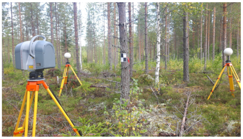
2. Mobile

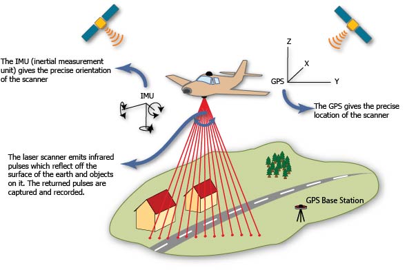
3. Airborne
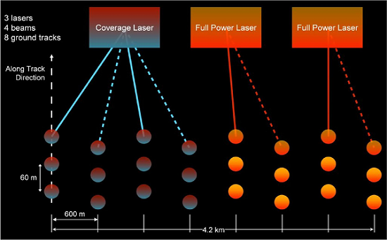
5. Satellite
The focus of the remainder of this exercise will be on airborne lidar.
That said, the information provided could be readily applicable to any discrete-return lidar system.
The most common format for discrete-return lidar point cloud data is a LAZ file (e.g., lidar_data.laz). LAZ files are a lossless compression of LAS files, which was the industry standard lidar data format for a long time. LAS files are still used somewhat, but given the vastly reduced file sizes of LAZ, LAZ has largely replaced LAS.
The standard file format for LAZ files can be found in the American Society of Photogrammetry & Remote Sensing’s LAS Specification guide. At their core, point clouds are simply tabular data with x, y, and z coordinates, along with a suite of other (potentially) useful attributes. I’ll highlight the most important ones you’re likely to use below:
There are many others, but these are the ones you are most likely to use.
In the US, the two best sources of airborne lidar data are The USGS 3D Elevation Program (3DEP) and OpenTopography. The USGS, of course, has a lengthy history of terrain mapping in the US with its production of topographic maps dating back to the late 19th century. Beginning in 2016, the USGS set about to collect airborne lidar over all of the contiguous US. Less than a decade later, the vast majority of the CONUS has been scanned:
It is worth noting that 3DEP has different nominal quality levels (QL):
| Quality Level | Vertical Accuracy RMSE | Nominal Pulse Spacing | Nominal Pulse Density |
|---|---|---|---|
| QL0 | 5 cm | <= 0.35 m | >= 8 pts/m2 |
| QL1 | 10 cm | <= 0.35 m | >= 8 pts/m2 |
| QL2 | 10 cm | <= 0.71 m | >= 2 pts/m2 |
Note that these are minimum standards – most USGS QL1 data, for example, has considerably higher pulse density than 8 pts/m2. Furthermore, the point density is always higher than this, given that pulses return multiple points (usually 1-4).
OpenTopography is an NSF-funded facility based at UC San Diego that ingests and serves up all of the USGS 3DEP data in addition to a variety of non-USGS lidar datasets (ALS, TLS, and photogrammetric point clouds). It also offers some basic but potentially very valuable data processing capacities, such as point cloud reprojection and derivation of raster products.
For what it’s worth, I typically get data directly from the USGS for a few reasons:
As with any dataset (especially spatial data), there is a multitude of software options for processing, analyzing, and viewing lidar point cloud data. I won’t even come close to listing them all, but I will point out a few that warrant mentioning.
1. LAStools
2. CloudCompare
3. Python (pdal)
pdal) and is built on the concept of building point cloud processing piplines using JSON syntax.4. R (lidR)
In this exercise, we will focus on using lidR in R to analyze lidar data.
For the purposes of this exercise, we will need some lidar data to play with. Please follow the instructions below to download a few tiles of lidar data.
Keep in mind that the goal of this exercise is to download four tiles of lidar data. The USGS typically tiles up its lidar data into 1 x 1 km boxes, so you should try (to the best of your ability) to draw a 2 x 2 km polygon. You will likely have to iterate on this several times before you get the scale right. You can feel free to download more tiles, but know that lidar data are quite large in size, and processing more tiles will not only require more storage capacity and memory, but also processing time.
We also want lidar tiles from the same “project”. The 3DEP program is sort of a hodgepodge of individual lidar data collection campaigns (or, “projects”) that are collected through local, state, and federal partnerships. Unfortunately this makes life a little complicated, as different projects are collected with different specifications, at different times, with different projections, etc. So, for the sake of this exercise, you’re going to want to download four tiles within the same project. You can tell they are a part of the same project based on the file names that are returned after clicking Search Products. They should all have the same prefix and Published Date. As you hover over them, their footprints will be highlighted on the map.
If you don’t want to bother with trying to identify the four, single-project, “perfect” lidar tiles for this exercise, then you can simply download the four example tiles used in this exercise. They cover the base and some of the lower ski runs at Alta Ski Area. You can access them here:
Now, onto the fun part! In this part of the exercise, we are going to open everyone’s favorite statistical software package (R!) and install all of the libraries necessary for the successful execution of the remainder of this exercise.
lidR’s functionality is dependent upon sf.lidR also depends heavily on terra.# install packages
install.packages("sf")
install.packages("terra")
install.packages("lidR")
install.packages("viridis")
install.pacakges("future")The next steps are to load the libraries we just installed (using the library() function) and read in our lidar data. There are two main ways to read in lidar data in lidR:
readLAS() allows you to read in a single LAS/LAZ file of lidar data.readLAScatalog() allows you to read in several tiles at once.The vast majority of the time, you will be relying on #2, as readLAScatalog() creates a LAScatalog object that enables parallel processing of several tiles at once, including an awareness of tile topology, which avoids edge artifact issues. For more on the LAScatalog class, please consult this vignette.
In the script editor, write code that accomplishes the following:
# load libraries
library(sf)
library(terra)
library(lidR)
library(viridis)
library(future)

# define directory structure
main_dir <- "C:/Users/u0942838/Documents/lidar_exercise"
lidar_dir <- file.path(main_dir, "lidar_data")
raw_dir <- file.path(lidar_dir, "a01_raw")
dtm_dir <- file.path(lidar_dir, "a02_dtm")
dsm_dir <- file.path(lidar_dir, "a03_dsm")
hgt_dir <- file.path(lidar_dir, "a04_hgt")
chm_dir <- file.path(lidar_dir, "a05_chm")
veg_dir <- file.path(lidar_dir, "a06_veg")
other_dir <- file.path(main_dir, "other_data")

# read in single tile of lidar data
tile_files <- list.files(
  path = raw_dir,
  pattern = "*.laz$",
  full.names = T
)
tile_file <- tile_files[1]
las <- readLAS(tile_file)
Attaching package: 'rmarkdown'The following object is masked from 'package:future':
runIn the example above, you’ll notice the use of the variable name las for the LAS object returned by the call to readLAS(). This might be a little confusing, since we’re using LAZ files (not LAS) files, but this is merely a naming convention used within the lidR ecosystem. You can, of course, feel free to name variables whatever suits your style, but know that all references henceforth will assume your data are stored as las.
Let’s do some data exploration:
# print las summary
las
class : LAS (v1.4 format 6)
memory : 1.6 Gb
extent : 445000, 446000, 4492000, 4493000 (xmin, xmax, ymin, ymax)
coord. ref. : NAD83(2011) / UTM zone 12N + NAVD88 height - Geoid12B (metre)
area : 1 km²
points : 20.96 million points
density : 20.96 points/m²
density : 15.29 pulses/m²This yields several valuable pieces of information, including the total (uncompressed) memory required to store these data, the spatial extent, the coordinate reference system, the total area covered by the tile, the number of points in the dataset, as well as the point (1st) and pulse (2nd) densities.
Next, let’s take a look at the attributes contained within the data. Underneath the hood of each LAS object, there is a data.table containing each point’s attributes. To access the table, you can use las@data.
# explore the attributes
las@dataNext, we’ll do some point cloud visualization. Depending on how big your file is and how capable your computer is, this next step may go better or worse. Visualizing point clouds is a fairly computationally (graphically) expensive procedure, given that you’re trying to visualize millions of points in 3D. But, let’s give it a shot! You can visualize point clouds using the plot() function.
# plot the point cloud out
plot(las)
Like any R plotting function, there are lots of ways to alter your data visualization by manipulating the parameters supplied to plot(). For a full accounting of them, you can enter ?lidR::plot().
# plot point intensity
plot(las, color = "Intensity", breaks = "quantile", nbreaks = 50)Lidar return intensity is theoretically a very interesting and useful variable. It measures how much of a laser’s pulse energy is returned to the sensor for a particular return. There are several factors that affect return intensity:
1. The reflective properties of the surface the pulse interacted with
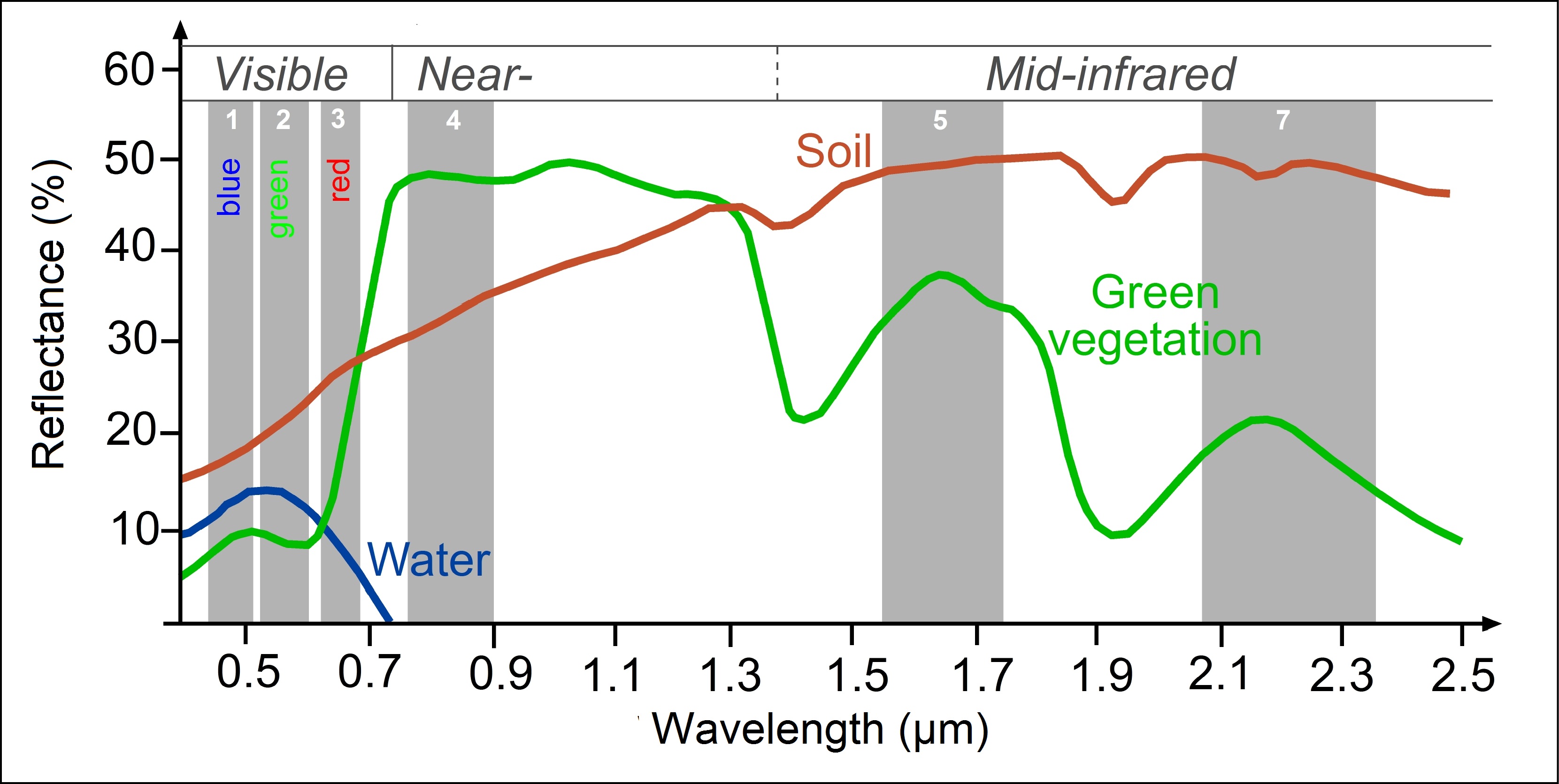
2. The geometric properties of the surface

3. The pulse angle
4. The lidar-surface range
5. Multiple returns

6. Sensor specifications
Taking all of that into consideration, this is why I have said that intensity is a theoretically interesting and useful metric. There are plenty of scientists using intensity to gain some understanding of surface type (in addition to merely surface position), but it’s a challenging pursuit!
If you’re using the point cloud data provided in this exercise, when you plot out the first point cloud, you will see that there are some erroneous points far above and below the true land surface. Unfortunately, noise points like these are not uncommon in discrete-return airborne lidar data. Fortunately, the USGS or the vendors who collected the data will typically run some processes to classify these points as noise, allowing users like us to filter them out. Looking back at the LAS Specification 1.4 (Table 17), we can see that there are two noise classes (7 and 18). Let’s use this as an opportunity to see the distribution of different classes in the Classification attribute of our point cloud data.
# summarize class totals
table(las$Classification)
       1        2        7       18
14915555 6028121 15119 91 Note that, when using the dollar sign approach for subsetting, you can access attributes in two different ways. You can do so using the las@data$Classification syntax, or you can simply use las$Classification. However, if you want to subset a column using brackets, you can only do so using the @data approach (e.g., las@data[,"Classification"]).
In the example data, it looks like some points have been pre-classified as both 7: Low Point (Noise) and 18: High Noise. Your dataset may not have these, but they should at least have classes 1 (Unclassified) and 2 (Ground). If not, you may reconsider using these data for the remainder of the exercise. It’s also worth noting that, when looking at Table 17 in the LAS Specification 1.4, there are many other classes (e.g., “Low Vegetation”, “Building”, etc.). Seeing this table gives the impression that lidar point clouds are regularly classified into these classes. The reality is that the vast majority of point clouds you download will only have classes 1, 2, 7, and 18 classified. You can certainly perform classifications yourself using several different approaches, but most point clouds are delivered in a somewhat “bare bones” fashion, given the challenge of accurately classifying billions of points.
Another attribute of interest that can sometimes be useful for removing bad data is the Withheld_flag. There seems to be a somewhat hazy distinction between noise points and withheld points, and most typically points that are classified as noise (i.e., either 7 or 18) will also be flagged to be withheld. But, there are instances in which they may not nest cleanly.
# tabulate withheld point flags
table(las$Withheld_flag)
   FALSE     TRUE
20943676 15210 # cross-tabular withheld flag with classification
table(las@data[,c("Withheld_flag", "Classification")]) Classification
Withheld_flag 1 2 7 18
FALSE 14915555 6028121 0 0
TRUE 0 0 15119 91In this case, all noise points are also withheld.
Knowing that we have some noisy data on our hands, we are now going to filter out those points in order to ensure that any products we derive from the point cloud data are as accurate as possible. Noise filtering is a fairly standard part of any lidar data processing workflow. There are two ways to remove points pre-classified as noise from your point cloud:
1. When loading the data (preferred)
filter argument in the readLAS() function.2. After the data are loaded (less preferred)
filter_poi() function.Technically both are viable, but the former is more efficient in that it never has to read the noisy points into memory as they are ignored entirely. So, let’s proceed with that approach.
# read in the data while filtering out noise
las <- readLAS(tile_file, filter = "-drop_class 7 18")

# tabulate classification
table(las$Classification)
       1        2
14915555 6028121 # plot the data out
plot(las)In the example data, there do not appear to be any obvious, remnant noise points after removing those already classified as noise (or flagged as withheld). However, if your data do appear to still have some noise (which is not uncommon!), you can do the following:
# run noise classification using statistical outlier removal (sor) algorithm
# with default parameters
las <- classify_noise(las, sor())

# remove those points
las <- filter_poi(las, !(Classification %in% c(7, 18)))
Note that lidR functions are well-suited to the tidyverse or native R pipe functions to streamline data pipelines and avoid repetitive code. The code above could be more clealy re-written as:
# run noise classification and filter out those points
las <- las |>
  classify_noise(sor()) |>
filter_poi(!(Classification %in% c(7, 18)))There are many situations in which it would be useful to have a spatial subset of your point cloud data. In fact, the odds that you are somehow magically interested exactly in the ambiguously defined 1 x 1 km grid format the data are delievered in are quite slim. One of the most common reasons you might want a spatial subset of data is if you have field plots within which some data were collected. To ensure spatial compatibility between the data collected in the field and the lidar data, you can clip the lidar data within the field plot(s). The lidR package has several clipping functions.
Let’s test a couple of these out. First, we’ll use clip_circle() to represent a scenario in which we have collected a circular plot representing forest structure and we are aiming to compare the measured structure with lidar metrics.
# get the extent of your data
e <- ext(las)

# generate random x and y coords
x <- runif(1, e[1], e[2])
y <- runif(1, e[3], e[4])

# clip 15m radius plot
las_plot <- clip_circle(las, x, y, 15)

# plot it out
plot(las_plot)
Now, let’s clip a transect to examine the ground point classification quality. This is also a fairly common practice, particularly in situations where you have had to perform your own ground point classification. As mentioned earlier, if you are acquiring data from an authoritative source such as the USGS, it is very likely that ground points have already been classified. However, if you are collecting your own lidar data, such as UAS, TLS, or MLS lidar, you will have to perform your own ground point classification. This can be accomplished using classify_ground(). For the sake of brevity, this exercise will not cover that function, but it exists!
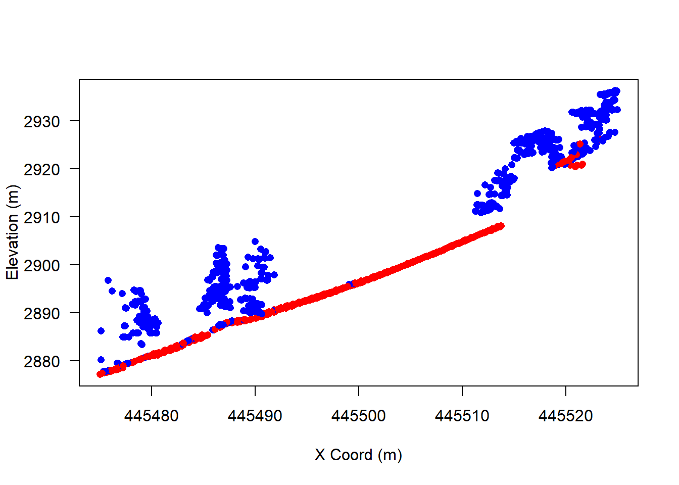
The goal of the next few steps is to examine a 50 m-long, 2 m-wide transect that is centered on the center point of your tile of lidar data, and runs directly along the x-axis of your data’s coordinate reference system (e.g., east-west).
# get the extent of your data
e <- ext(las)

# get the extent center point
x_center <- mean(e[1:2])
y_center <- mean(e[3:4])

# get the transect end point x coordinates
x_left <- x_center - 25
x_right <- x_center + 25
p1 <- c(x_left, y_center)
p2 <- c(x_right, y_center)

# clip the transect data
las_transect <- clip_transect(las, p1, p2, 2)

# get colors
col <- rep("blue", nrow(las_transect))
col[las_transect$Classification == 2] <- "red"

# plot it out in 2D
plot(
  x = las_transect$X,
  y = las_transect$Z,
  col = col,
  pch = 16,
  xlab = "X Coord (m)",
  ylab = "Elevation (m)",
  las = 1
)
Without a doubt, one of the most important functions of airborne lidar data is to enable the production of precise and accurate digital terrain models (DTMs). You may be more familiar with the term digital elevation model (DEM). And then there are also digital surface models (DSMs). Here is a quick clarification of terminology:

Indeed, the production of nationwide, high-resolution DTMs is the foremost objective of the USGS 3DEP. Quite simply, the production of a DTM from an airborne lidar point cloud involves the spatial interpolation of ground points. Thus, it is imperative that you have ground points classified prior to generating a DTM. Theoretically, any spatial interpolation algorithm could be used to generate a DTM, but the lidR library has implemented three algorithms within their rasterize_terrain() function:
knnidw(): k-nearest neighbor inverse distance weighting interpolation.tin(): triangulated irregular network interpolation.kriging(): Kriging interpolation.Of the three, tin() is by far the simplest computationally and, perhaps as a result, seems to be the most common approach across lidar processing software. However, it is the most subject to noise, as each ground point is fit to the TIN prior to gridding. Thus, if any ground points are misclassified, they will be represented in your final DTM. The other two methods may be somewhat more robust to erroneous data, but are more computationally expensive and may, in fact, yield an overly-smooth DTM if not properly tuned.
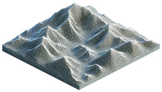
For those unfamiliar, a TIN is a vector-based, 3D representation of a surface of some sort (e.g., terrain elevation), where points are connected by a series of non-overlapping triangles. To derive a rasterized DTM from a TIN, the rasterize_terrain() function simply overlays a pixel grid on top of the TIN, extracts TIN elevations within each pixel. It’s not clear from the documentation, but my suspicion is that it simply takes the TIN value from the pixel’s center point. By default, if you have terra installed, lidR::rasterize_*() functions will return a terra::SpatRaster object.
# generate a dtm
dtm <- rasterize_terrain(las)

# check out its summary
dtm
class : SpatRaster
dimensions : 1000, 1000, 1 (nrow, ncol, nlyr)
resolution : 1, 1 (x, y)
extent : 445000, 446000, 4492000, 4493000 (xmin, xmax, ymin, ymax)
coord. ref. : NAD83(2011) / UTM zone 12N (EPSG:6341)
source(s) : memory
name : Z
min value : 2535.891
max value : 2991.812 # plot it out in 2D
plot(dtm)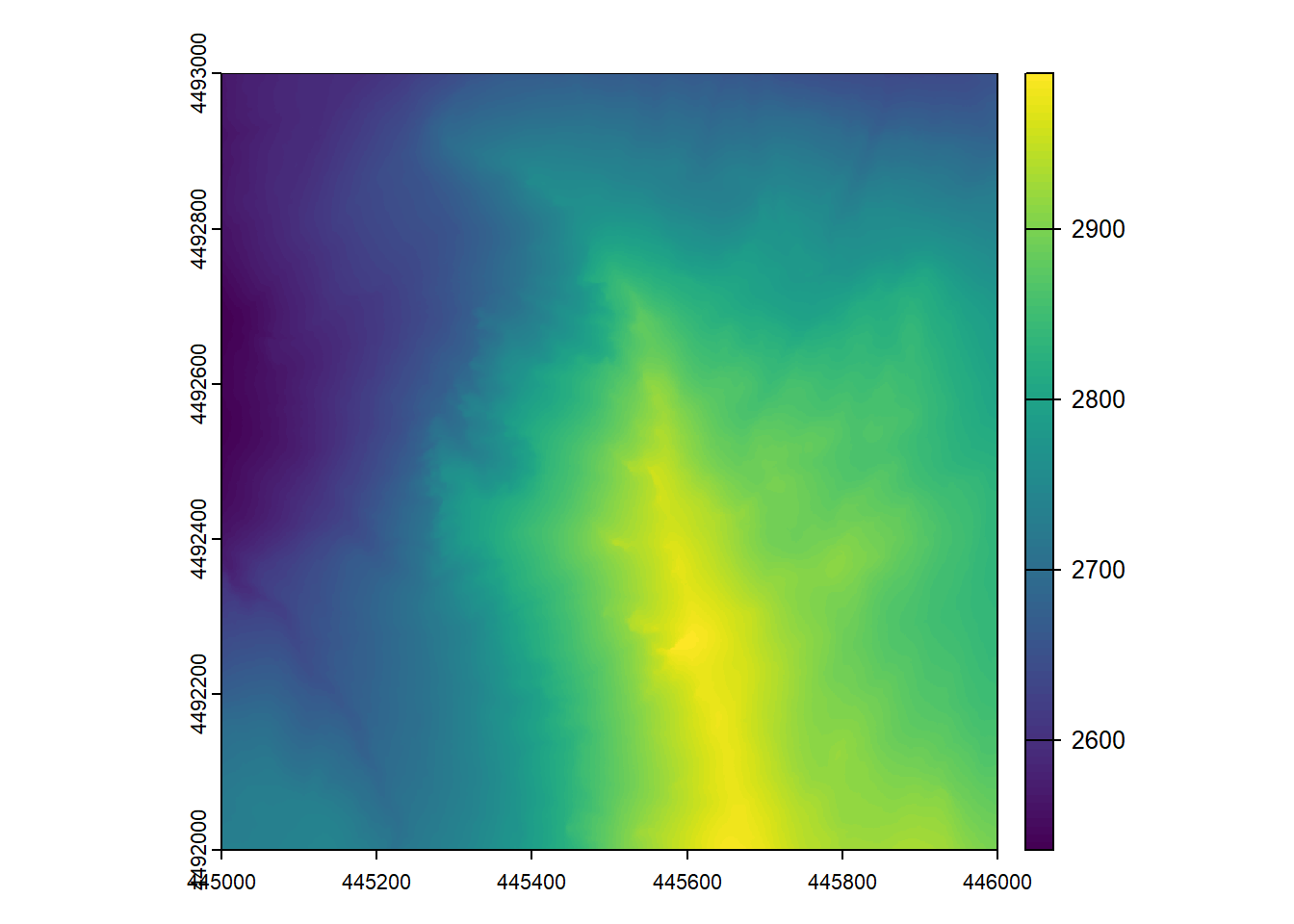
# plot it out in 3D
plot_dtm3d(dtm)
At this point, your DTM only lives in memory – that is, as soon as you close your R session, it will no longer exist. It is common practice when generating derivative products from lidar point cloud data to save the outputs to disk so that you do not have to repeat the same steps each time you might want to use the resulting DTM. In terra, this can be accomplished using the writeRaster() function. If you need to read the raster back into memory, you can do so using rast().
# write dtm to file
writeRaster(dtm, file.path(lidar_dir, "dtm.tif"), overwrite = T)

# read it back in
dtm <- file.path(lidar_dir, "dtm.tif") |> rast()
Of course, there is an immense number of cool things you could do with the resulting DTM, but for the sake of brevity, we’ll leave those up to your imagination.
The process for generating a DSM mirrors that for DTMs in almost every way. There are two main differences:
Instead of interpolating a raster surface from ground points, the interpolation is based on all first return points. This ensures that the resulting raster represents the elevation of the highest (sampled) surface above the ground. If there are no aboveground features (e.g., trees, buildings), then the ground surface elevation will be represented in the DSM (i.e., DTM == DSM).
The function for generating a DSM in lidR is rasterize_canopy(). It is a bit of a confusing nomenclature (“why not rasterize_surface()?”), but it makes some sense, because you apply the same function to generate a canopy height model when supplying it with ground height-normalized point cloud data. More on this later. rasterize_canopy() has three algorithms implemented:
p2r(): simple “point to raster” approach, where raster values are assigned the highest single point elevation.
dsmtin(): triangulated irregular network interpolation.
pitfree(): a modified version of p2r() that tries to remedy the gaps (or “pits”) that can emerge when interpolating a canopy surface.
For the sake of simplicity, let’s stick with dsmtin() for now. We will explore the others later on.
There is no plot_dsm3d() function, but you can use plot_dtm3d(), even if the input is a DSM and not a DTM. Sometimes you’ve got to break the rules. Live a little.
# generate a dsm
dsm <- rasterize_canopy(las, algorithm = dsmtin())

# check out its summary
dsm
class : SpatRaster
dimensions : 1000, 1000, 1 (nrow, ncol, nlyr)
resolution : 1, 1 (x, y)
extent : 445000, 446000, 4492000, 4493000 (xmin, xmax, ymin, ymax)
coord. ref. : NAD83(2011) / UTM zone 12N (EPSG:6341)
source(s) : memory
name : Z
min value : 2536.650
max value : 3001.567 # plot it out in 2D
plot(dsm)
# plot it out in 3D
plot_dtm3d(dsm)

# write dsm to file
writeRaster(dsm, file.path(lidar_dir, "dsm.tif"), overwrite = T)

# read it back in
dsm <- file.path(lidar_dir, "dsm.tif") |> rast()
If you’ve used the exercise data, and you look closely, you should be able to see some “lumps” of higher elevation on top of the previously-plotted DTM. Of course, those are trees.
DTMs are inherently useful for a wide range of terrain mapping applications. DSMs are somewhat less commonly used, but still have some useful functions. More useful than a DSM is a normalized digital surface model (nDSM), representing surface heights above the ground. In a forest, this is also known as a canopy height model (CHM). Note that I will use nDSM and CHM interchangeably throughout this exercise, as the example dataset represents a largely forested area. The simplest way to derive an nDSM is by subtracting the DTM pixel values from the DSM pixel values. terra makes this process trivial – all basic mathematical functions can be applied directly to SpatRaster objects (as long as they align spatially in extent, resolution, origin, and coordinate reference system).
# generate ndsm
ndsm <- dsm - dtm

# plot it out in 2D
plot(ndsm)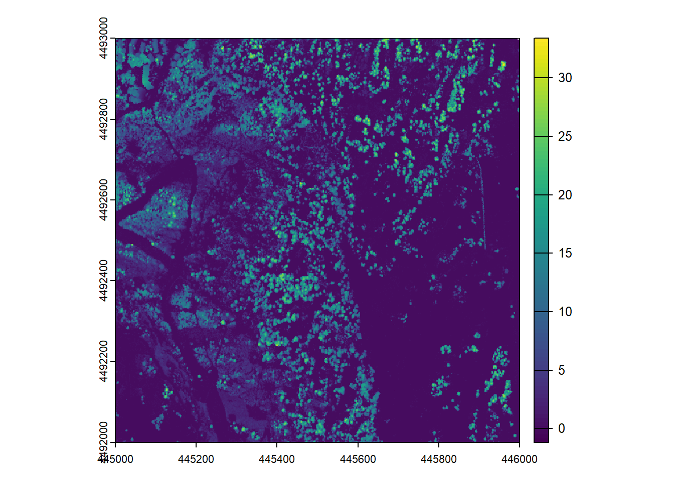
# plot it out in 3D
plot_dtm3d(ndsm)

# write ndsm to file
writeRaster(ndsm, file.path(lidar_dir, "ndsm.tif"), overwrite = T)

# read it back in
ndsm <- file.path(lidar_dir, "ndsm.tif") |> rast()The keen-eyed may have noticed the previous section’s title alluding to the fact that there are multiple approaches for generating a nDSM/CHM. Depending on your needs, there is an argument to be made that the approach just described (DSM - DTM = nDSM) is the lesser of approaches, as it is potentially more subject to an erroneous output. A more nuanced approach for generating a potentially more accurate nDSM is by height-normalizing your point cloud data. In effect, this converts lidar point elevations (e.g., in meters above mean sea level) to lidar point heights (e.g., in meters above the ground). Beyond the potentially minor quality differences between an nDSM derived from DSM-DTM subtraction versus interpolation of a height-normalized point cloud, there are many situations in which it is inherently useful to have height-normalized lidar point cloud data. For example, if you are aiming to model vegetation structure using a suite of vegetation structural predictor variables derived from lidar data, you will need height-normalized data to accomplish that task.
In lidR, height normalization is accomplished using the aptly named normalize_height() function. When examining this function’s arguments (i.e., entering ?normalize_height), it should look very similar to those from a function you previously ran: rasterize_terrain(). That is because underneath the hood, they are doing the very same thing – interpolating ground points to create an approximation of the ground surface. The difference between rasterize_terrain() and normalize_height() is that the latter takes it one step further by subtracting the ground surface elevation from each lidar point. Note that the function also contains an argument dtm to which you can actually supply a DTM SpatRaster, which will be the basis of ground subtraction. Although more efficient, the same terrain elevation is subtracted from all points that fall within a given pixel, which can lead to, in effect, a “stair-step” type of uncertainty, particularly in steep environments. So, if accuracy and precision are of primary interest, this approach is generally not favored.
# normalize heights
las_hgt <- normalize_height(las, tin())

# plot it out
plot(las_hgt)Now we’re going to repeat what we did a few steps ago – generating an nDSM – except this time we’re going to use our new, height-normalized point cloud data. Furthermore, we’re going to test out three different algorithms for interpolating an nDSM and visually compare them for quality.
# generate ndsm using dsmtin(), write to file, and read back in
ndsm_dsmtin <- rasterize_canopy(las_hgt, algorithm = dsmtin())
out_file <- file.path(lidar_dir, "ndsm_dsmtin.tif")
writeRaster(ndsm_dsmtin, out_file, overwrite = T)
ndsm_dsmtin <- rast(out_file)

# generate ndsm using p2r() and write to file
ndsm_p2r <- rasterize_canopy(las_hgt, algorithm = p2r())
out_file <- file.path(lidar_dir, "ndsm_p2r.tif")
writeRaster(ndsm_p2r, out_file, overwrite = T)
ndsm_p2r <- rast(out_file)

# generate ndsm using pitfree() and write to file
ndsm_pitfree <- rasterize_canopy(las_hgt, algorithm = pitfree())
out_file <- file.path(lidar_dir, "ndsm_pitfree.tif")
writeRaster(ndsm_pitfree, out_file, overwrite = T)
ndsm_pitfree <- rast(out_file)

# get spatial subset for plotting
e <- ext(las_hgt)
x_center <- mean(e[1:2])
y_center <- mean(e[3:4])
x_min <- x_center - 25
x_max <- x_center + 25
y_min <- y_center - 25
y_max <- y_center + 25

# set up plot
par(mfrow = c(1,3))

# plot the data out
plot(
  ndsm_dsmtin,
  xlim = c(x_min, x_max),
  ylim = c(y_min, y_max),
  main = "dsmtin"
)
plot(
  ndsm_p2r,
  xlim = c(x_min, x_max),
  ylim = c(y_min, y_max),
  main = "p2r"
)
plot(
  ndsm_pitfree,
  xlim = c(x_min, x_max),
  ylim = c(y_min, y_max),
  main = "pitfree"
)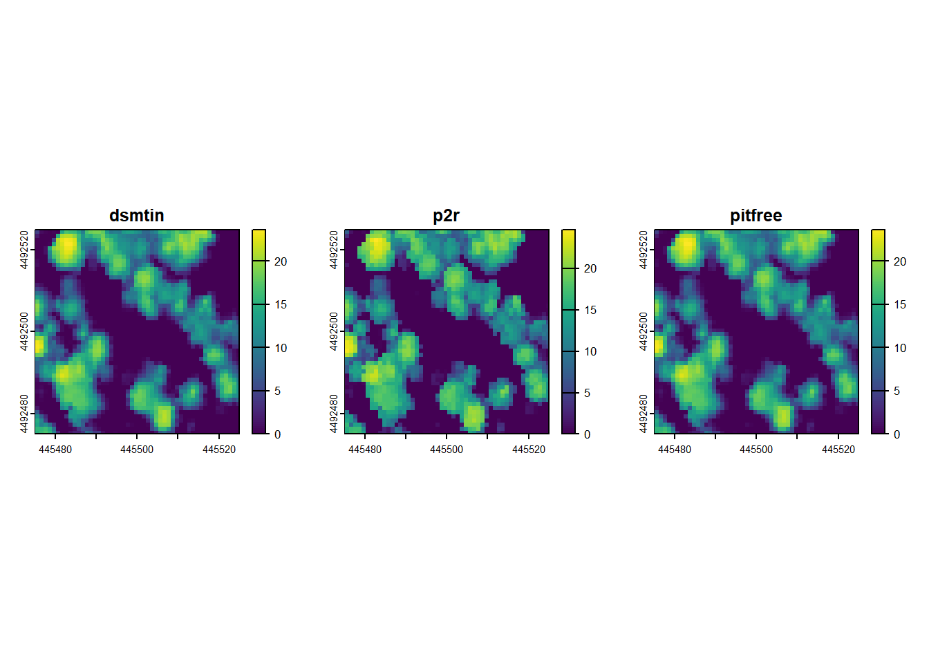
The differences between the three nDSMs are no doubt subtle, but a careful examination reveals that both dsmtin() and pitfree() yield comparably smoother-looking tree crowns than p2r(). Depending on your needs, that smoothness may be considered an advantage (e.g., if you aim to perform some tree crown delineation procedure) or a disadvantage (e.g., if you aim to retain tree structure, noise and all). Although this exercise dataset does not demonstrate this phenomenon very well, both dsmtin() and p2r() can yield many “pits”, where lidar pulses have been able to exploit small gaps in the canopy, and first returns reflect off of lower portions of the canopy, understory vegetation, or even the ground. Here is an example of that:

Here is an example of a “pitfree” version of the same dataset:

Accordingly, I generally prefer to use the pitfree() algorithm when generating nDSMs/CHMs to ensure both an aesthetically pleasing and analytically sound dataset.
There are two primary analytical paradigms in airborne lidar-based analysis of vegetation structure:

In this section, we will focus on #1. In the next section, we will focus on #2. The lidR function for computing area-based structural metrics is pixel_metrics(). If you enter ?pixel_metrics, not only will you see the parameters needed for executing that function, you will see a host of other *_metrics() functions within lidR that operate in a very similar manner. All of them hinge on the supply of a user-defined function to the argument func. These functions can range from exceedingly simple to extremely complex. There are a few considerations when creating these functions:
pixel_metrics(), each item in that list will yield a raster dataset. So, if you list has two metrics, you will produce a 2-layered raster dataset, where pixels in each layer represent the metric defined by the function.~) when supplied to the func parameter. For example, if you had a function named cr_mets(), and it had one argument z, you would supply that to crown_metrics() like func = ~cr_mets(Z).func = ~cr_mets("Z") would fail, for example.This is described in much greater detail in the lidR book, but hopefully this is enough information to get you started.
# function for mapping mean and maximum height
f <- function(z){
  list(
    mean_z = mean(z),
    max_z = max(z)
  )
}

# apply function to generate 10m map of mean and max height
r <- pixel_metrics(las_hgt, ~f(Z), 10)

# plot it out
plot(r)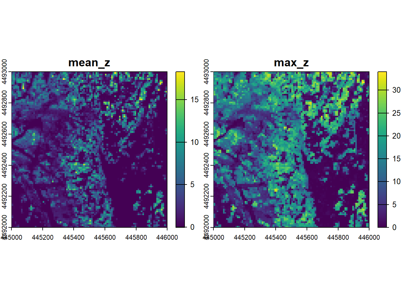
# function for mapping canopy cover
f <- function(z, r){
  z <- z[r == 1]
  numer <- length(z[z >= 2])
  denom <- length(z)
  cc <- numer / denom
  l <- list(cc = cc)
  return(l)
}

# apply function to generate 10m map of canopy cover
r <- pixel_metrics(las_hgt, ~f(Z, ReturnNumber), 10)

# plot it out
plot(r)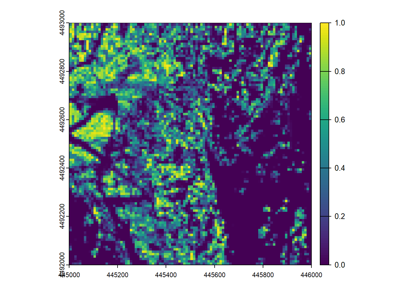
This map (hopefully) represents the proportion of returns that intercepted the canopy relative to all returns, therefore representing the proportional canopy cover.
One of the really cool things you can do with height-normalized lidar point cloud data is delineate individual tree crowns. This assumes, of course, that your lidar dataset covers an area that features trees, which our exercise dataset does. By now I feel like a parrot when I say “there are many algorithms that can be employed…”, but I must once again repeat this statement. When delineating tree crowns, there are a host of different algorithms one could use. In fact, there are hundreds (thousands?). If you enter “delineate tree crowns from airborne lidar” into Google Scholar, you will see 15k+ results at the time this exercise was written. Thankfully, the lidR library has incorporated a limited (but still diverse) set of tree crown delineation algorithms, giving you a useful degree of constrained flexibility.
In lidR, tree crown delineation is really a two-step process:
1. Detecting tree tops
2. Delineating crowns
The lidR book does a great job of walking through this procedure and evaluating the effects of different approaches. For the sake of this much more cursory exercise, we will step through a singular workflow to achieve a hopefully desirable (though certainly imperfect!) result.
Let’s begin by subsetting our point cloud to a smaller area. Tree crown delineation can be a fairly computationally expensive process, so working within smaller areas (especially for testing purposes) can be highly beneficial. Furthermore, visually interpreting the outputs is much easier when viewing a local area rather than an entire 1 km2 tile of lidar data.
# get spatial subset for clipping
e <- ext(las_hgt)
x_center <- mean(e[1:2])
y_center <- mean(e[3:4])
x_min <- x_center - 50
x_max <- x_center + 50
y_min <- y_center - 50
y_max <- y_center + 50

# clip height-normalized lidar data
las_clip <- clip_rectangle(
  las_hgt,
  x_min,
  y_min,
  x_max,
  y_max
)In a perfect world, you would know exactly where all of the tree tops are located within an area of interest. If you are working within relatively small field plots, it is conceivable that you could measure tree top point locations on the ground using a high-accuracy GPS. However, that is not a very scalable solution. So we are often left to rely on automatic tree top detection approaches. In lidR, this is accomplished using a moving window approach, using one of two window types:
1. Fixed-diameter
2. Dynamically sized
In lidR, the function for identifying tree tops is locate_trees() and the algorithm you supply to it for parameterizing your moving window is lmf().
We need a height-to-crown width function to supply to lmf(). We could, of course, make one up. For example, we could assume that trees are generally 5x taller than their crown width. Of course, that depends highly on species and setting. In our region, for example, juniper trees can often be as wide as they are tall (i.e., crown width = 1 x tree height). Conversely, subalpine fir trees can have extremely narrow crowns (i.e., crown width = 0.1 x tree height). Knowing the species composition of your study area may be highly beneficial for generating a locally calibrated local maximum filter.
To that end, let’s take a look at TALLO: a global tree allometry and crown architecture database. We will plot out and attempt to model crown width as a function of tree height using species that are known to be in our example study area.
# read in the tallo data
df_tallo <- file.path(other_dir, "Tallo.csv") |> read.csv()

# subset to just species of interest
sp <- c(
  "Abies lasiocarpa", # subalpine fir
  "Abies concolor", # white fir
  "Populus tremuloides", # quaking aspen
  "Pseudotsuga menziesii", # Douglas-fir
  "Picea engelmannii", # Engelmann spruce
  "Picea pungens" # blue spruce
)
df_tallo <- df_tallo[df_tallo$species %in% sp,]

# subset to just dry western us
df_tallo <- df_tallo[
  df_tallo$latitude >= 30 &
    df_tallo$latitude <= 50 &
    df_tallo$longitude <= -100 &
    df_tallo$longitude >= -120,
]

# remove rows without necessary data
df_tallo <- df_tallo[
  complete.cases(df_tallo[,c("height_m", "crown_radius_m")]),
]

# compute crown diameter
df_tallo$crown_diameter_m <- df_tallo$crown_radius_m * 2

# get point colors by density
dc <- densCols(
  x = df_tallo$height_m,
  y = df_tallo$crown_diameter_m,
  colramp = colorRampPalette(c("black", "white"))
)
df_tallo$pt_dens <- col2rgb(dc)[1,] + 1L
df_tallo <- df_tallo[order(df_tallo$pt_dens),]
cols <- viridis(256)
df_tallo$col <- cols[df_tallo$pt_dens]

# plot crown radius versus height
plot(
  crown_diameter_m ~ height_m,
  data = df_tallo,
  pch = 16,
  col = df_tallo$col,
  xlab = "Tree Height (m)",
  ylab = "Crown Radius (m)",
  las = 1
)

# fit linear model
mod <- lm(crown_diameter_m ~ height_m, data = df_tallo)
mod_x <- range(df_tallo$height_m)
mod_y <- predict(mod, newdata = list(height_m = mod_x))
lines(mod_y ~ mod_x, col = "hotpink", lwd = 3)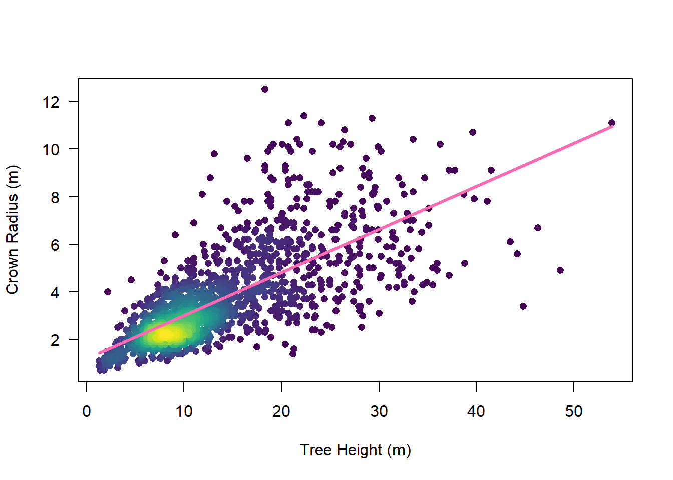
# get linear model summary
summary(mod)
Call:
lm(formula = crown_diameter_m ~ height_m, data = df_tallo)

Residuals:
    Min      1Q  Median      3Q     Max
-5.9125 -0.7542 -0.2119  0.6048  7.9881

Coefficients:
            Estimate Std. Error t value Pr(>|t|)
(Intercept) 1.196729   0.072554   16.49   <2e-16 ***
height_m    0.181155   0.004609   39.30   <2e-16 ***
---
Signif. codes:  0 '***' 0.001 '**' 0.01 '*' 0.05 '.' 0.1 ' ' 1

Residual standard error: 1.387 on 1485 degrees of freedom
Multiple R-squared:  0.5099,    Adjusted R-squared:  0.5096
F-statistic:  1545 on 1 and 1485 DF,  p-value: < 2.2e-16
It’s definitely not a perfect linear correlation, but the model explains over half of the variance in crown radius, so it’s a much better starting point than a random guess! For the example data, this yields the following local maximum filter function:
\[d = 0.2z + 1.2\]
where \(d\) is the crown diameter and \(z\) is the tree height, both in meters. We can now translate this into an R function that can be fed to lmf() which, in turn, can be fed to locate_trees() to identify treetops in our study area.
# create lmf function
f <- function(z) {0.2 * z + 1.2}
l <- lmf(f, 2, "circular")

# identify treetops
ttops <- locate_trees(las_clip, l)

# plot it out in 3D
x <- plot(las_clip, bg = "white", size = 4)
add_treetops3d(x, ttops)
Looks pretty good!
Now that we have our treetop seed points, we can feed those into one of several segmentation algorithms. Tree segmentation is the process by which points in a cloud (and/or pixels in a CHM) are assigned to (classified by) the tree to which they most likely belong. It is an imperfect but very useful procedure, especially when tree structural variables (e.g., height, biomass, etc.). One of the reasons it is imperfect is because most segmentation algorithms, including those included in lidR, tend only to be good at segmenting overstory trees – that is, the trees whose crows can be seen from above. Understory trees are likely to be missed or lumped into the segment of tree crowns that overtop them.
To see all of the tree segmentation algorithms available in lidR, you can enter ?segment_trees. Feel free to explore them each on your own, but for the sake of this exercise, we will use dalponte2016(). The algorithm is described in Dalponte & Coomes (2016). It is a region-growing algorithm that iteratively associates pixels surrounding the treetop points to each tree according to a few rules defined by the parameters th_tree (minimum tree height), th_seed (region growing parameter 1), th_cr (region growing parameter 2), and max_cr (the maximum crown diameter).
Before segmenting trees in the example dataset, however, we are going to have to first generate a new CHM that matches the extent of our clipped point cloud data, since the previous CHM was generated from the full tile of data.
# generate 25cm chm
chm_trees <- rasterize_canopy(las_clip, 0.25, pitfree())

# segment tree crowns
las_trees <- segment_trees(las_clip, dalponte2016(chm_trees, ttops))

# plot in 3d by tree id
plot(las_trees, color = "treeID")
At least in the example dataset, the default segmentation parameters yielded subpar results, with lots of points being left unclassified. This is likely due to the high spatial resolution of the CHM and the fact that max_cr is based on number of pixels. Let’s run again with a much larger max_cr value to hopefully yield an improved delineation.
# generate 25cm chm
chm_trees <- rasterize_canopy(las_clip, 0.25, pitfree())

# segment tree crowns
las_trees <- segment_trees(
  las_clip,
  dalponte2016(
    chm = chm_trees,
    treetops = ttops,
    max_cr = 50
  )
)

# plot in 3d by tree id
plot(las_trees, color = "treeID")
A marked improvement, no doubt. But still clearly imperfect. There are many different approaches one could take to automate and assess the effects of delineation algorithm parameters, but doing so is beyond the scope of this exercise. Feel free to play with the parameters some more if you desire a better delineation. For the sake of the remainder of this exercise, we’ll stick with this delineation, and see what fun things we can do with it.
Using the previously delineated trees, we can derive some useful structural metrics for each tree in your area of interest. This is extremely useful for forest ecology (understanding forest structure over space), fire ecology (understanding fuel structure over space), forestry (quantifying merchantable timber), and even carbon accounting (deriving tree-level carbon estimates through allometry). It could even be used to help create a training database for a machine learning model that attempts to map some structural parameter over large areas – a task that can be very arduous to do manually.
In lidR, this is accomplished very simply using the crown_metrics() function. This function returns an sf object, either POINT or POLYGON depending on the user-defined geom of interest. As discussed in a previous section, the *_metrics() functions in lidR allow you to summarize point cloud data within some geometry of interest – in this case, tree crown polygons. For crown_metrics(), you can choose several different geometries, including point(single point for each delineated tree),convex(convex hull around delineated trees),concave(concave hull), andbbox` (bounding box).
# define a function for summarizing tree structure
f <- function(z){
  list(max_z = max(z))
}

# get tree polygons
crowns <- crown_metrics(
  las = las_trees,
  func = ~f(Z),
  geom = "concave"
)

# examine the crowns sf polygon object
crowns
Simple feature collection with 196 features and 2 fields
Geometry type: POLYGON
Dimension: XY
Bounding box: xmin: 445450 ymin: 4492450 xmax: 445550 ymax: 4492550
Projected CRS: NAD83(2011) / UTM zone 12N + NAVD88 height - Geoid12B (metre)
First 10 features:
treeID max_z geometry
1 3 8.384 POLYGON ((445498.3 4492546,...
2 4 20.811 POLYGON ((445501.4 4492540,...
3 5 22.397 POLYGON ((445502.6 4492530,...
4 6 19.933 POLYGON ((445494 4492547, 4...
5 7 16.701 POLYGON ((445496.9 4492534,...
6 8 19.754 POLYGON ((445498.7 4492531,...
7 9 22.936 POLYGON ((445501 4492526, 4...
8 10 14.102 POLYGON ((445502.7 4492520,...
9 11 20.290 POLYGON ((445505.5 4492515,...
10 12 18.496 POLYGON ((445504.8 4492507,...If you are not familiar with the sf library, it is a world unto itself well worth your exploration time at some later date. For now, we’ll use it in a very basic way – to plot out the tree crowns and their associated heights in 2D. Take a quick look here to learn how to do that: https://r-spatial.github.io/sf/articles/sf5.html.
# plot out
plot(crowns["max_z"])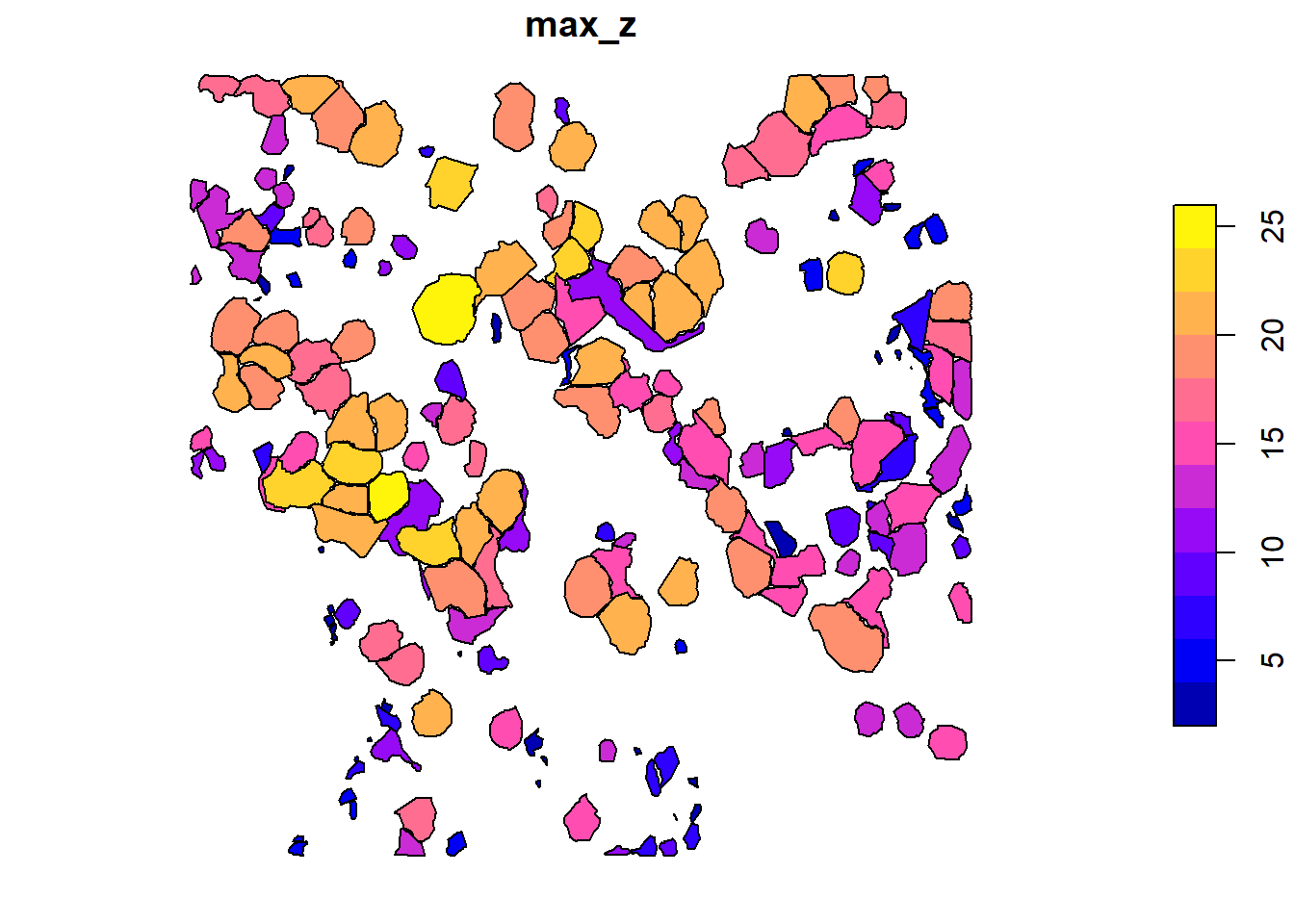
By now you’re probably asking yourself “why did I download four tiles of lidar data when all we’ve processed so far is one?!” You would be right to ask that question, and your fury is completely justified. But rage no more, my friend, because you have now arrived at this exercise’s final destination: the LAScatalog.
LAScatalog is an awesome object type in lidR that allows users to apply the same set of functions to a set of lidar tiles, rather than operating on each tile separately. The entire package is designed so that nearly any function applied to a LAS object can also be applied to a LAScatalog object, and vice versa. Not only that, but they allow for parallel processing of your lidar tiles, which can considerably speed up your data processing, especially if you are working with a large extent. Furthermore, they are designed with tile topology in mind, with built-in buffering capability that ensures that there will be no edge effects in landscape products derived from tiled lidar data. The vast majority of the time you are working with lidar data, you are all but certain to be working with LAScatalog objects more than LAS objects, because tiling is the industry standard for data delivery and you need computational solutions that treat tiles as parts of a whole, rather than meaningful units unto themselves.
To read your point cloud data in as a LAScatalog, you can use the readLAScatalog() function. Like its single-tile counterpart, readLAS(), readLAScatalog() allows you to select a subset of columns or filter to a refined set of points. Unlike its counterpart, you can supply the function’s folder argument with the file directory in which your tiles are stored.
# read in the lascatalog data
ctg <- readLAScatalog(raw_dir, filter = "-drop_class 7 18 -drop_withheld")

# examine it
ctg
class : LAScatalog (v1.4 format 6)
extent : 445000, 447000, 4492000, 4494000 (xmin, xmax, ymin, ymax)
coord. ref. : NAD83(2011) / UTM zone 12N + NAVD88 height - Geoid12B (metre)
area : 4 km²
points : 75.22 million points
density : 18.8 points/m²
density : 14.5 pulses/m²
num. files : 4 # plot it out
plot(ctg)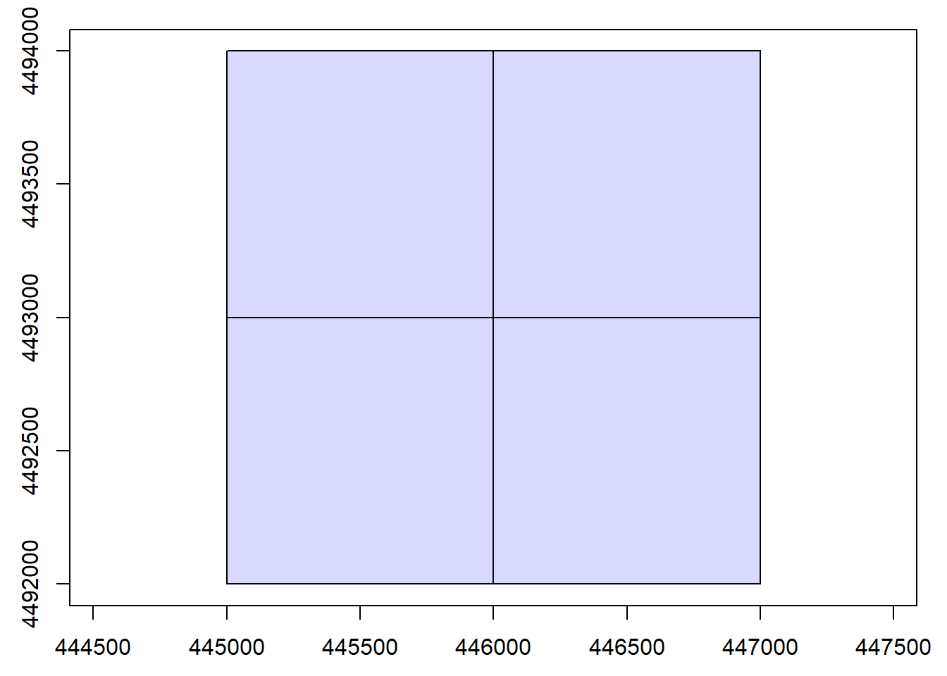
One of the things that makes LAScatalogs so powerful is their inherent awareness of topology. Knowing which tiles, and which points within those tiles, are adjacent to points in neighboring tiles allows for seamless analysis of tiled data. This topology is created through spatial indexing. First introduced by LAStools, the spatial indexing system for LAS/LAZ data involves the creation of LAX files. These are very small files that can be rapidly generated for each LAS/LAZ file in a directory that efficiently store point locations through a quadtree-based position encoding system. You can read in and process LAScatalogs without LAX files, but (as noted in the lidR book) processing efficiency is considerably reduced.
So, the question is: how do we generate LAX files? Interestingly, lidR does not have its own indexing function. Instead, it suggests using LAStools to generate these indices. As an alternative, it points to a function in the rlas library, which is a major dependency of lidR, written by the same author, that contains some lower-level functions. Among those functions is writelax(), which allows you to generate a spatial index (LAX) file for a single input LAS/LAZ file.
# geneate lax files
raw_files <- list.files(raw_dir, pattern = "*.laz$", full.names = T)
for (raw_file in raw_files){
  rlas::writelax(raw_file)
}

# read in your lascatalog again
ctg <- readLAScatalog(raw_dir, filter = "-drop_class 7 18 -drop_withheld")LAScatalog processing optionsThere are several options that you may need to manipulate while working with LAScatalogs. You can see the full list by entering ?"LAScatalog-class" into the console. Below I will highlight a few that you are most likely to employ:
1. chunk_size:
LAScatalogs’ topology, you can actually process “chunks” (i.e., pseudo-tiles) of any dimensions. This is particularly handy if you are working on a computer that does not have a lot of RAM, and/or are working with extremely large point cloud files. In situations like these, you could define smaller chunks than the original tile dimensions, allowing less data to be read in at once during processing.opt_chunk_size(ctg) <- x, where ctg is your LAScatalog object and x is the length and width of the chunk in the units of the data’s coordinate reference system.2. buffer:
opt_chunk_buffer(ctg) <- x, where ctg is your LAScatalog object and x is the buffer size in the units of the data’s coordinate reference system.3. laz_compression:
FALSE) or LAZ files (TRUE).opt_laz_compression(ctg) <- x, where ctg is your LAScatalog object and x is either TRUE (or T) or FALSE (or F).4. output_files:
LAScatalog. For example, if you are generating a DTM from many chunks/tiles, you may want to store each chunk/tile’s DTM in a file directory. This avoids having to store all of that data in memory, allowing you to subsequently read the tiled DTMs in (as a terra::vrt, for example) from disk.opt_output_files(ctg) <- x, where ctg is your LAScatalog object and x is a file path template used to name the output files. There are a few template options:
# directory structure
in_dir <- "c:/raw_lidar_data"
out_dir <- "c:/dtms"

# read data in
ctg <- readLAScatalog(in_dir)

# set output files
opt_output_files(ctg) <- file.path(out_dir, "{ORIGINALFILENAME}")

# generate dtms, saving each tile
rasterize_terrain(ctg)
In the example above, if in_dir had two tiles (“tile_1.laz” and “tile_2.laz”), the successful execution of this script would yield two DTM tiles in out_dir (“tile_1.tif” and “tile_2.tif”).
Note that there are other LAScatalog processing options that some lidR users might interact with (e.g., stop_early, alignment, drivers), but those are beyond the scope of this high-level overview. If you can familiarize yourself with the syntax and logic of setting a few of these processing options, you can easily figure out how to set others.
futureAs mentioned earlier, LAScatalogs allow for efficient data processing through parallelization. As described in the documentation when you enter ?"lidR-parallelism" into the console, lidR allows for two different types of parallelization:
1. Algorithm-based parallelization
set_lidr_threads(x), where x is the number of cores you want to use.2. Chunk-based parallelization
multisession using the future library.# set up multisession with 5 workers (i.e., employ 5 CPU cores)
plan(multisession, workers = 5L)
# read in your data
ctg <- readLAScatalog(in_dir)
# run some process
dtm <- rasterize_terrain(ctg)
# end multisession
plan(sequential)In both of these cases, it is important to be cautious about balancing CPU usage with RAM. For example, if you have 10 cores on your machine, you may be tempted to employ all of them in a chunk-based parallelization. But, if each of the chunks contains 5GB of data, this would require 50GB of RAM, as lidR reads entire chunks in at once.
Now, let’s pull all of this to the test!
In the code snippet below, you will see the following line in several places:
ctg@output_options$drivers$SpatRaster$param$overwrite <- T
This mess of code is specifically designed to ensure that, if the script is run multiple times, it will not return an error when trying to write individual raster tiles (DTM, DSM, CHM, and CC) to files.
# begin parallelization
plan(multisession, workers = 2L)

# read in lascatalog
ctg <- readLAScatalog(raw_dir, filter = "-drop_class 7 18 -drop_withheld")

# generate dtm
opt_output_files(ctg) <- file.path(dtm_dir, "{ORIGINALFILENAME}")
ctg@output_options$drivers$SpatRaster$param$overwrite <- T
dtm <- rasterize_terrain(ctg)
Chunk 1 of 4 (25%): state ✓
Chunk 2 of 4 (50%): state ✓
Chunk 3 of 4 (75%): state ✓
Chunk 4 of 4 (100%): state ✓writeRaster(dtm, file.path(lidar_dir, "dtm.tif"), overwrite = T)
# generate dsm
opt_output_files(ctg) <- file.path(dsm_dir, "{ORIGINALFILENAME}")
ctg@output_options$drivers$SpatRaster$param$overwrite <- T
dsm <- rasterize_canopy(ctg, algorithm = dsmtin())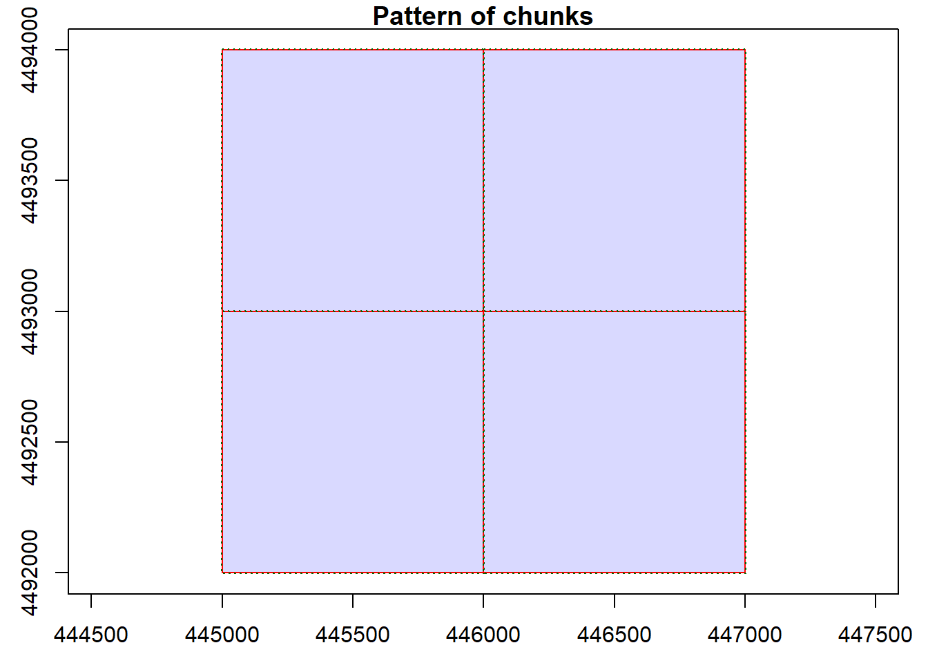
Chunk 2 of 4 (25%): state ✓
Chunk 1 of 4 (50%): state ✓
Chunk 3 of 4 (75%): state ✓
Chunk 4 of 4 (100%): state ✓writeRaster(dsm, file.path(lidar_dir, "dsm.tif"), overwrite = T)
# normalize heights
opt_output_files(ctg) <- file.path(hgt_dir, "{ORIGINALFILENAME}")
opt_laz_compression(ctg) <- T
normalize_height(ctg, tin())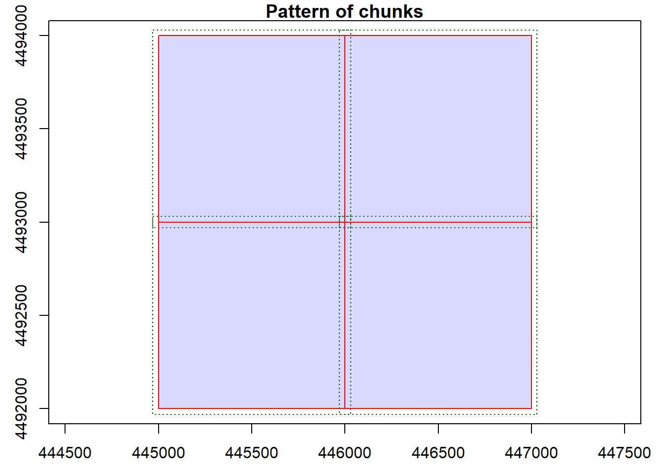
Chunk 2 of 4 (25%): state ✓
Chunk 1 of 4 (50%): state ✓
Chunk 3 of 4 (75%): state ✓
Chunk 4 of 4 (100%): state ✓
class : LAScatalog (v1.4 format 6)
extent : 445000, 447000, 4492000, 4494000 (xmin, xmax, ymin, ymax)
coord. ref. : NAD83(2011) / UTM zone 12N + NAVD88 height - Geoid12B (metre)
area : 4 km²
points : 75.16 million points
density : 18.8 points/m²
density : 14.5 pulses/m²
num. files : 4 # generate canopy height model
ctg_hgt <- readLAScatalog(hgt_dir, filter = "-drop_class 7 18 -drop_withheld")
opt_output_files(ctg_hgt) <- file.path(chm_dir, "{ORIGINALFILENAME}")
ctg_hgt@output_options$drivers$SpatRaster$param$overwrite <- T
chm <- rasterize_canopy(ctg_hgt, algorithm = pitfree())
Chunk 2 of 4 (25%): state ✓
Chunk 1 of 4 (50%): state ✓
Chunk 3 of 4 (75%): state ✓
Chunk 4 of 4 (100%): state ✓writeRaster(chm, file.path(lidar_dir, "chm.tif"), overwrite = T)
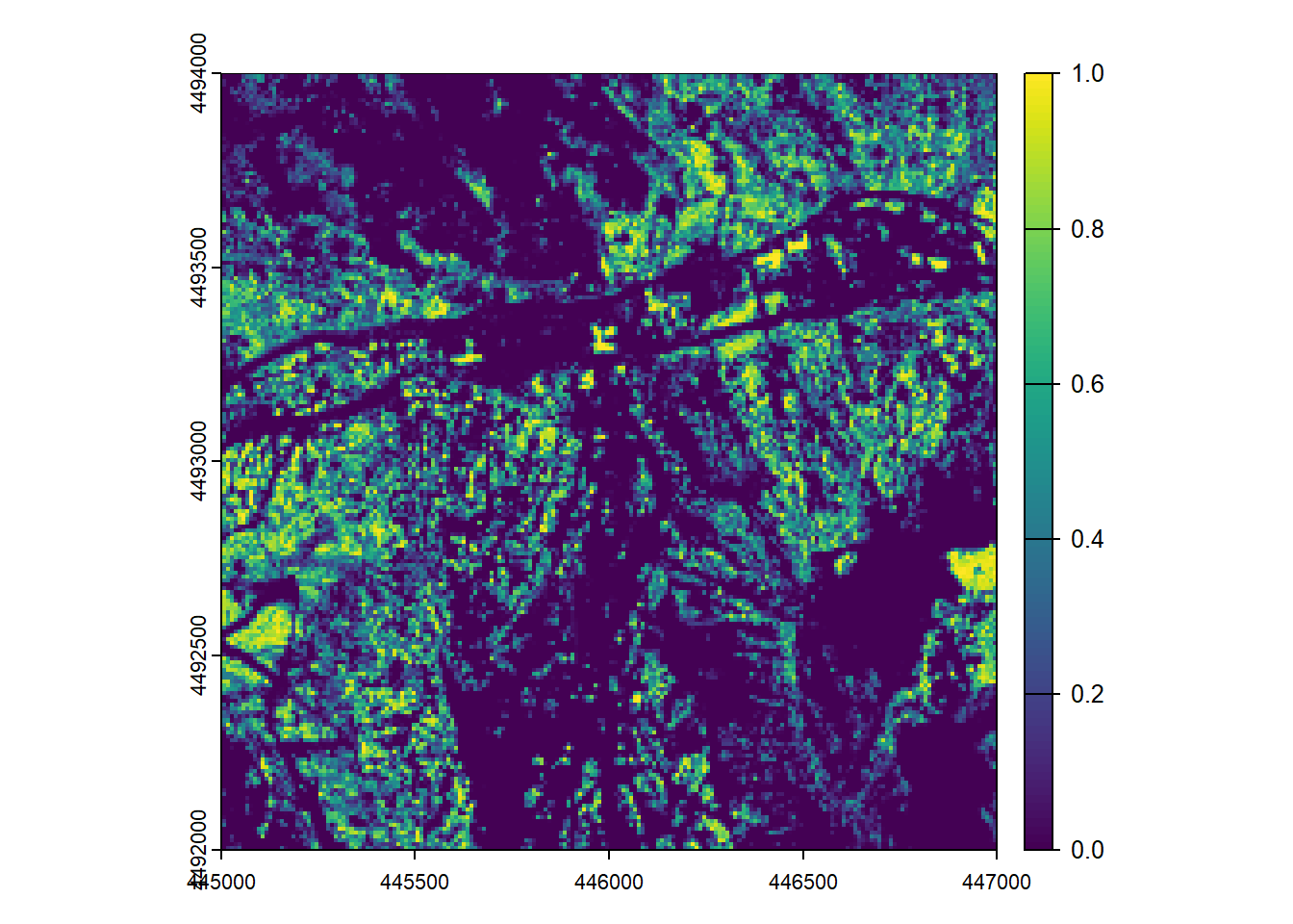
# generate canopy cover raster
f <- function(z, r){
z <- z[r == 1]
numer <- length(z[z >= 2])
denom <- length(z)
cc <- numer / denom
l <- list(cc = cc)
return(l)
}
opt_output_files(ctg_hgt) <- file.path(veg_dir, "{ORIGINALFILENAME}")
ctg_hgt@output_options$drivers$SpatRaster$param$overwrite <- T
cc <- pixel_metrics(ctg_hgt, ~f(Z, ReturnNumber), 10)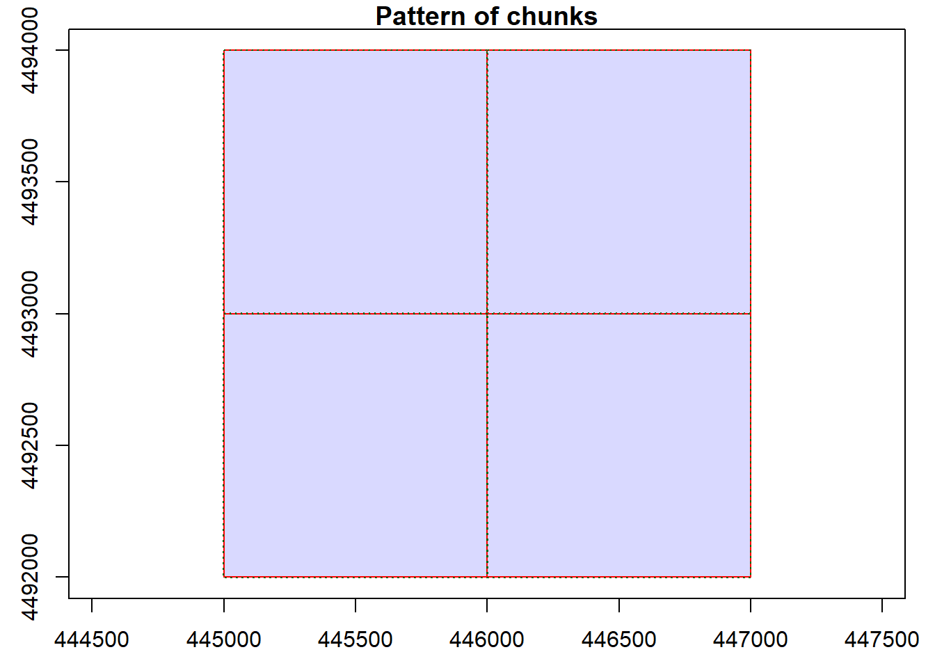
Chunk 2 of 4 (25%): state ✓
Chunk 1 of 4 (50%): state ✓
Chunk 3 of 4 (75%): state ✓
Chunk 4 of 4 (100%): state ✓writeRaster(cc, file.path(lidar_dir, "cc.tif"), overwrite = T)
# end parallelization
plan(sequential)
# read them back in
dtm <- file.path(lidar_dir, "dtm.tif") |> rast()
dsm <- file.path(lidar_dir, "dsm.tif") |> rast()
chm <- file.path(lidar_dir, "chm.tif") |> rast()
cc <- file.path(lidar_dir, "cc.tif") |> rast()
# plot outputs
plot(dtm)
plot(dsm)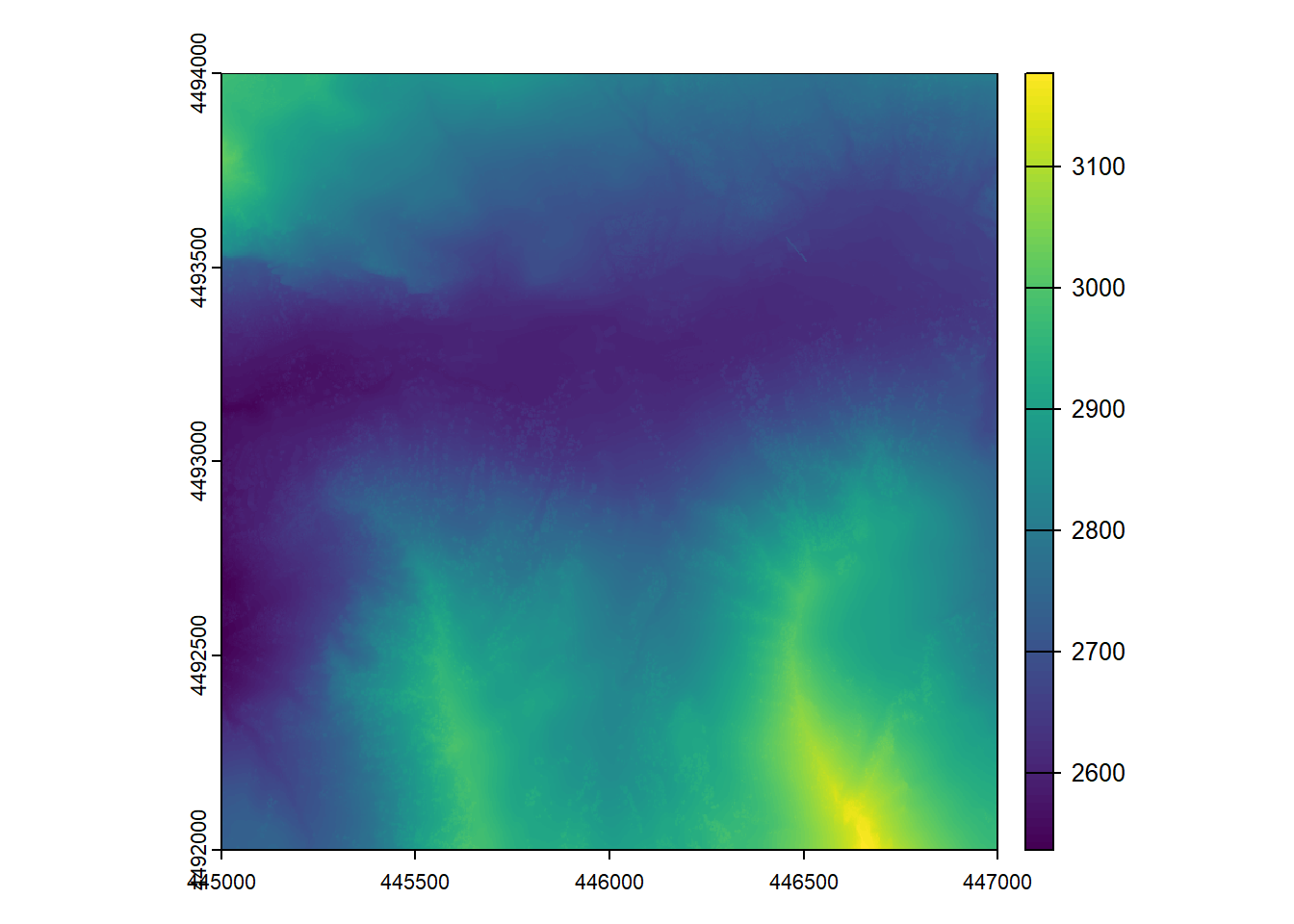
plot(chm)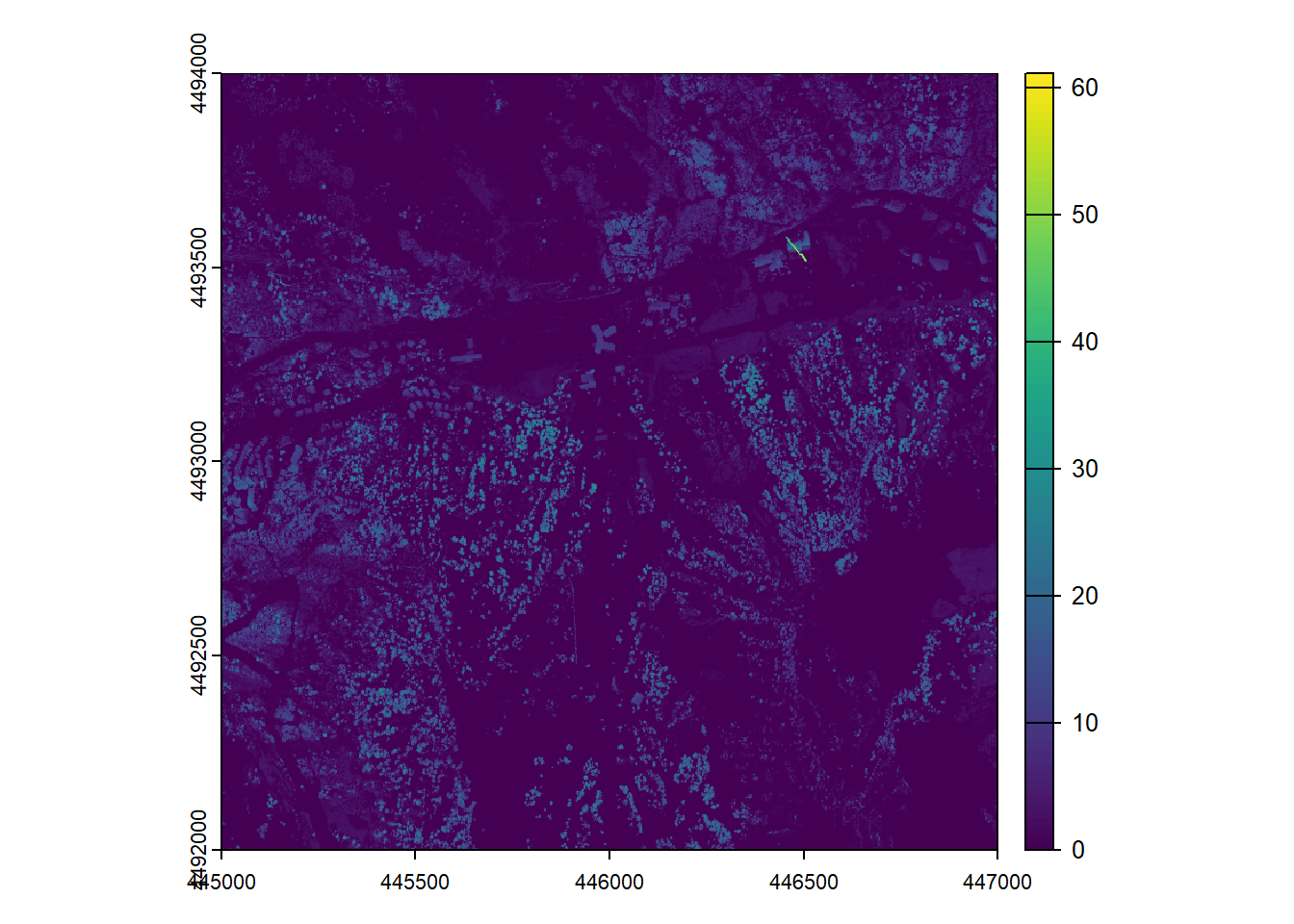
plot(cc)